Deep Double Descent in Large Language Models: A Unified View of Grokking

Gaining insights into the behavior and performance of large language models (LLMs) is undoubtedly one of the intricate challenges in modern AI research. Deep double descent and the grokking phenomenon intricately reveal the model optimization and generalization process, which is far from straightforward. This blog post aims to richly integrate these two phenomena through the lens of large-scale training paradigms.

In this article, I am going to provide a blend of theories and beliefs about those ‘magic moments’ when model performance starts to increase after non-monotonically correlating with model parameters or data volume with deep double descent and when the model can generalize well after being exhaustively trained on sparsely populated datasets, a process dubbed as grokking. This article motivates and guides the thinking about those elusive model behaviors and their implications in the context of rational large-language model design and deployment. This post seeks to capture the underlying processes of these powerful forces defining modern AI model development, from the details of the mechanisms involved to practical solutions.

What is Double Descent in Large Language Models?

The term “double descent” relates to a peculiar observation made of the majority of models used in machine learning, especially the large language models (LLMs), where the generalization error decreases following a model inversion \textit{-} which occurs at the augmentation of the model size or greater complexity of training set. The double descent that appears in machine learning derives its name from the type of error plot it creates and can usually be decomposed into distinct phases. In LLMs, double descent is commonly attributed to the interactions of model capacity, data complexity, and the training process. This further illustrates that existing paradigms on overfitting and underfitting have gaps, positing that over-parameterized models yield excellent performance when well-trained. This behavior must be deeply understood for optimal model and training strategy design.

Understanding the Double Descent Phenomenon

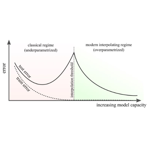
Double descent is a model’s generalization performance following a U-shaped curve that declines after what is traditionally deemed the point of overfitting. Classical models have faced a trade-off between bias and variance. Still, over-parameterized models—models with more parameters than training data—tend to lessen this trade-off to achieve peak performance. This is because with significant increases in the model size comes the ability to capture essential patterns in the data and minimize critical noise. Being familiar with this behavior and proper regularization techniques is imperative to aid in using double descent for better and more precise predictive model designs.

How Double Descent Differs from Traditional Learning Curves

Double descent challenges the learning curves by providing a new perspective on model effectiveness. As with more traditional learning curves, models driven by double-descent learning typically show a steady decline in errors as they become more complex. This means the addition of parameters or any other form of complexity enhances the model until it adequately captures the data to the point of overfitting, which leads to errors beyond a specific limit.

Mistakes can go back down – Take note of this crucial detail regarding the double descent curve. The range of complexity within the model can reach a level where it is exceedingly overfitted, yet errors can decrease. This can be attributed to the communication between the underparameterized and overparameterized regimes.

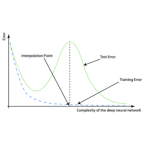
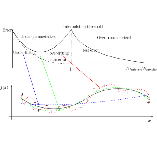
Underparameterized Regime:

This is where the model has not built enough capability to capture the data's complexity fully.
Both training and test errors are high.

Interpolation Threshold:

The complexity midpoint where model complexity is equal or slightly greater than the training data.
This results in the model perfectly fitting the training data. However, this leads to overfitting and a test error peak.

Overparameterized Regime:

Model complexity goes beyond the interpolation threshold.
Surprisingly, the test error decreases due to the model's enhanced ability to depict varying data patterns through low and high parameter counts.

Key Technical Parameters:

Model Complexity, seen as the depth of neural networks or the number of their parameters, increases performance in the double descent curve
For a given model, performance is optimal when overparameterized and sufficiently regularized.
Regularization Techniques:
Applying dropout, weight decay, or early stopping helps reduce error and stabilizes learning.
Data Size:
Increased data lowers the peak at the interpolation threshold, lessening the severity of double descent.

This phenomenon reshapes our understanding of model generalization; overparameterization can leverage data in superior ways. This is important in contemporary machine learning, especially with highly overparameterized models like neural networks.

The Relationship Between Double Descent and Overfitting

Double descent disputes the traditional concept of overfitting by illustrating that exceeding a model's complexity beyond the interpolation threshold does not abandon generalization; in fact, it can improve upon it. Overfitting usually means poor performance on new data due to excessive attention being given to the training set. Still, double descent showcases a secondary improved performance phase as model capacity increases. This accentuates that careful observation of data and model architecture in an overparameterization scenario like neural networks can reduce overfitting, transforming it into a resource for better learning results.

When Does Deep Double Descent Occur in Neural Networks?

Deep double descent is commonly seen in neural networks during the model's shift from an underparameterized state to an overparameterized state. At first, an increase in model capacity results in overfitting, leading to worse generalization. After a certain number of parameters are reached, performance improves once more, achieving generalization due to the model’s greater flexibility in solution fitting. This is common when training large datasets with complex architectures, emphasizing the dynamic dependency between model size, dataset scale, and optimization.

Model-Wise Double Descent: Impact of Number of Parameters

About the impact of model-wise parameters, the double descent phenomenon states that performance does not reduce proportionally alongside overfitting. The concept exists that when parameters are added to the model, it causes delays or worsens the model's performance with overfitting. Once a specified region is surpassed, the parameters enable the model to delve deeper into the solution space, explore it freely, optimize alongside numerous additional parameters, and enhance performance. This explains the complex relations among model architecture, data complexity, and optimization methods.

Epoch-Wise Double Descent: The Role of Training Time

Epoch-wise double descent pertains to the phenomenon whereby a model’s performance (in terms of generalization error) improves during a training session but worsens temporarily as an overfitting stage begins to set in until it improves once again with more training. This behavior is perplexing, underscoring the relationship between model sophistication, time spent in training, and generalization.

The main contributor leading to epoch-wise double descent is the transition from underfitting to overfitting and finally to effective generalization. In the early epochs, the model learns several patterns from the data, gradually decreasing the training and validation errors. However, as the training proceeds past a certain point (depending on the dataset and model architecture), overfitting begins to set in, causing an increase in validation error, even as the training error continues to decline. After this overfitting phase, the model is allowed to start exploring; convergence to a model that generalizes from the training set causes a first phase of error reduction.

Technical Parameters to Note:

Learning Rate (0.001-0.01): A low learning rate can prevent overshooting during prolonged training phases and facilitate the achievement of a good solution.
Epochs (50-500): The larger the dataset, the more training epochs are usually needed to reach the specific threshold for double descent.
Batch Size (e.g., 32-256): Lesser batch sizes can help strike a computation-efficient balance in discovering better minima.
Model Complexity (parameters): More parameterized networks display double descent behavior more dominantly because they are more likely to overfit, followed by generalization.
Regularization Techniques: Dropout (e.g., 0.2-0.5) or weight decay (e.g., 1e-4 to 1e-5) techniques can control overfitting and alter the double descent timing.

One must carefully adjust these parameters to balance generalization and model stability throughout prolonged training to comprehend and take advantage of epoch-wise double descent.

Data-Wise Double Descent: When More Data Can Hurt Performance

In a double descent scenario, model performance worsens after an initial improvement as the size of the training dataset increases. This occurs due to the model's inability to manage extra complexity introduced with additional data, which can only counter it when the dataset size reaches a certain threshold. The model adapts better to the underlying patterns as the dataset grows, resulting in improved generalization. The key takeaway is that additional data is not always beneficial, and clever and robust modeling techniques are required to avoid these issues while curating the data.

Why Do Larger Models Show Different Double Descent Patterns?

The expression of overfitting and regularization results in more complex patterns of double descent for larger models due to their capacity to resolve complex data distributions coupled with their ability to fit diverse datasets. Such models tend to overfit to smaller or noisy datasets first and then easily uncover complex patterns in larger datasets, which is why they perform better. This further highlights the relationship between model complexity, data size, and regularization when optimal generalization is the aim.

The Paradox of Bigger Models and Generalization

Generalization becomes paradoxical with larger models owing to the tradeoff between capacity and robustness. I believe larger models with more parameters can often generalize better because they can represent more complex functions. However, this depends on appropriately regularized training and significant amounts of it. Inadequate amounts can result in overfitting, where noise is captured rather than meaningful patterns. A few, but not all, important parameters to think about comprise the number of layers, their width (neurons per layer), and dropout or weight decay regularization. As does the batch size, schedule-dependent learning rate modulation also depends, which affects the updates' volatility. To circumvent overfitting or underfitting, it is critical that these parameters, given the dataset’s size and complexity constraints, are met appropriately to ensure optimal performance.

How Model Size and Training Data Interact

The relationship between model size and training data is crucial in any learning algorithm. Models with a larger number of parameters and features can capture complex patterns; however, these models also necessitate a large volume of quality training data to ensure effective generalization and mitigate overfitting. On the other hand, smaller models can work reasonably well with less training data, but their ability to model complex or large datasets is often significantly limited.

When building a model and mapping it to the training data, take into account the following settings:

Number of Parameters: Large models (for millions of examples, tens of millions of parameters) and small models (for small datasets, thousands of parameters).
Regularization: Apply L2 weight decay or dropout 0.2-0.5 to large models to avoid overfitting when working with smaller datasets.
Dataset Augmentation: Enrich the smaller datasets by using augmentation techniques such as flipping, rotation, or scaling.
Batch Size: Start with 32 or 64, depending on the model size and memory.
Learning Rate: Set mid-range learning rates with Adam optimizer (1e-3) and adjust with schedulers as needed.
Epochs: Use early stopping to prevent over-training and monitor performance on validation data to set epoch numbers.

Ultimately, scaling model size alongside the quantity and intricacy of training data is essential to attain dependable and effective model performance.

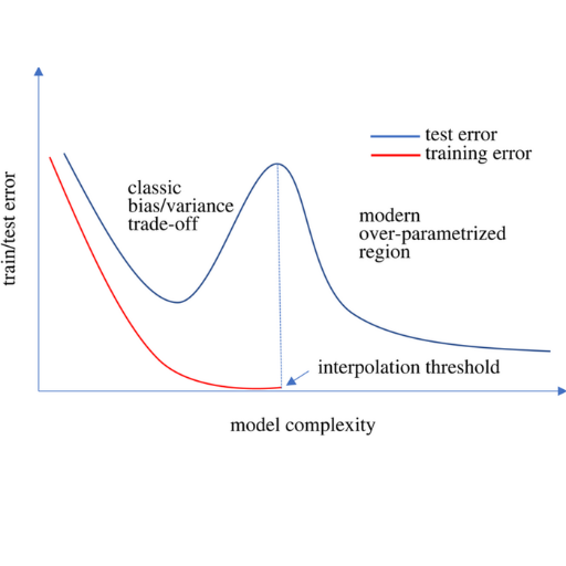
Double Descent in Deep Neural Networks vs. Traditional Models

Double descent describes the difference between classical models and deep neural networks in performance with increased model capacity. Traditional models tend to obey the bias-variance tradeoff; they suffer from high training errors due to excessive complexity, but overfitting deteriorates their performance on the test results. However, traditional deep neural networks have a peculiar trait: they have a reduction in test error referred to as ‘second descent’ beyond the interpolation threshold, showing that the models with even higher capacity do test better.

Key elements of the thesis scope are:

Model Capacity

Advanced deep learning networks feature a fixed polynomial degree of a particular layer and the parameters given to the model.
With deep neural networks, the radius of the layer, the number of nodes in the layer, and the number of parameters redefine the model's capacity.

Dataset Size

Large corpi of data are required so that deeper, later learning can take advantage of the benefits of the so-called second descent.
In contrast, the traditional model underrepresents a class of high-dimensional data in cases where the dataset is limited in size.

Regularization

Such models depend exclusively on regressions such as Lasso or Ridge.
In deep learning, some other ways to reduce overfitting are used: dropout, weight decay, and batch normalization.

Training Epochs

Both have limitations in avoiding unnecessary training and tend to use early stopping combined with validation monitoring or develop a system that is too complicated.

Through these distinctions, researchers can optimize deep learning performance and balance traditional methods by properly adjusting models and maximizing double descent.

Grokking and double descent are connected in their concern with generalization in deep learning. Grokking describes a model achieving an understanding of some patterns or capabilities after a training phase with low training error, often requiring long training times and specific conditions. This goes hand in hand with double descent, as both phenomena describe how overparameterized models can achieve better generalization. Examining grokking helps researchers understand why models show unexpected improvements, which is part of studying the double descent dynamics.

The Unified View of Grokking and Double Descent

The integrated view of grokking and double descent suggests that both rely on the model's capacity, its training, and the structure of data for building their model. Both instances are abundant in overparameterized models that possess sufficient capacity to capture complex patterns instead of only interpolation. In the case of grokking, prolonged training usually demonstrates enhanced generalization, precisely when small datasets are combined with regularization techniques such as weight decay or learning rate schedules. Analogously, double descent further emphasizes the capability of potent models to generalize effectively after reaching the interpolation threshold.

Corresponding Technical Parameters:

Model Capacity:

Overparameterization is crucial, meaning that the model has an overwhelmingly high number of parameters relative to the size of the data, which is not ideal.
Architecture examples consist of large transformer models or deep neural networks.

Training Time:

Grokking requires extensive training measured in epochs that far exceed typical convergence values (100-1000 epochs).
Validation loss and accuracy improve late in the training cycle and disallow the model to develop fully.

Regularization:

Weight decay is required to keep the model in check and prevent it from strongly overfitting (typical values range from 0.01 to 0.0001).
Training may be stabilized using dropout or gradient clipping.

Learning Rate Schedule:

Adaptive schedules commonly assist in grokking, while Cosine Annealing or warm restarts may improve double dissipation’s behaviour.

Characteristics of Dataset:

Small or organized datasets that have underlying patterns are ideal for witnessing grokking.
The application of double descent is seen across almost all data scales and complexities, but the improvement of generalization is quite distinct among large and varied datasets.

Because certain technical attributes of both ideas align, this framework provides direction to researchers attempting to understand the sophisticated ramifications of generalization within machine learning systems.

How Models Learn Through the Second Descent

I think models undergo a second descent while learning due to over-parameterization and pattern recognition in complex datasets. At first, as the model begins to memorize training data, the generalization performance becomes stagnant or begins to decline. In the second descent, further training improves the model’s prior learning processes so that it is able to capture broader patterns rather than simply memorizing data. This leads to better performance on new data.

Some critical parameters that affect this include:

Model capacity and architecture – relative to other models, over-parameterized models with greater capacity tend to exhibit the double descent phenomenon more profoundly.
Regularization techniques – appropriate use of L2 regularization or dropout increases generalization while decreasing overfitting.
Training duration: Prolonged training almost always aids the second descent, but this needs to be controlled to avoid convergence problems.
Learning rate schedules – adjusting the learning rate over time ensures the model functions as intended.
Dataset complexity – relatively large and varied datasets allow the model to distinguish between noise and valuable signals.

Adjusting these parameters can help us better understand and exploit the second descent in machine learning systems.

Distinguishing Between Grokking and Double Descent

Grokking and double descent are two phenomena of double nature in machine learning that are deeply connected. Grokking explains “overfitting” as a model achieving a perfect generalization after going through a lengthy training process, irrespective of the outcome produced at the onset of the model output. Double descent, conversely, explains the phenomenon where model performance dips after a specific capacity or training has reached a point where performance improvements can be made. Both concepts have particular features of overfitting and generalization, and the groping emphasizes learning over time. At the same time, double descent focuses on how model complexity and the data fed into the model fit.

What Practical Implications Does Double Descent Have for Training Language Models?

Practitioners should note that double descent argues that more care needs to be given to replicating already constructed language models due to the interplay between model performance and the model’s capacity in any task. Increasing the complexity of the model or extending the training periods may bring adverse outcomes at first, but these practices could potentially be rewarding. They should attempt to use bigger models or set more extended training periods to capture optimum performance even when these models contradict normal expectations. On top of that, double descent underlines a need for better data to permit lower performance without suffering from poor generalization to guarantee that the language model is accurate and competent.

Optimal Model Complexity for Different Dataset Sizes

Model complexity intricately correlates with the level of the dataset available alongside its volume. In particular, simpler models work best for smaller datasets, as they are less likely to overfit and can generalize well. In contrast, for larger datasets, complexity increases, and more powerful models that utilize the available data to fit complex patterns without overfitting the data become the most appropriate choice.

However, extreme model complexity heavily depends on the available computational resources. More powerful models require extensive memory and time alongside the appropriate hardware. Given this, validation and experimentation are the best solutions to determining the optimum complexity for the dataset at hand.

Strategies to Leverage Double Descent When Training Models

In utilizing double descent in model training, I try to balance model complexity and the size of the dataset. Smaller models are less likely to underfit when the training dataset is large enough, and I can take full advantage of overparameterization. With the large models, overgeneralization techniques such as L2 regularization and dropout are also necessary to gain additional control while improving generalization.

The learning rates and batch sizes are also very important. For example, I know that starting with a learning rate of 0.001 allows for optimal convergence, so I start there and monitor performance before adjusting. Training is guaranteed to pay the most dividend in double descent generalization when paired with monitoring validation performance and setting stopping times. Last, I have found that modifying the model architecture with the training schedule creates the most leverage in fully unleashing double descent generalization.

Key Technical Parameters:

Model size (e.g., number of layers or parameters): It should be proportionately aligned to the dataset to avoid underfitting and overfitting.
Learning rate: Start from 0.001, adjust accordingly.
Batch size: More often than not, 32-256, hardware and dataset dependant.
Regularization: Employ L2 regularization (e.g. λ=0.01) or dropout (e.g. rate=0.2).
Early stopping: Monitor validation loss and suspend training if improvement ceases.

As with many approaches, testing and flexibility are crucial to success with these strategies.

When Bigger Models and More Data Improve Performance

Based on my experience, tasks that involve complex identified patterns or large amounts of data, such as Natural Language processing or image recognition, work exceptionally well with larger models and extensive datasets. Larger datasets offer a wider range of data to learn and capture deep and intricate relationships for better generalization. Regularization, efficient training, and incorporating high-quality additional data are essential for improved productivity, alongside avoiding the pitfalls of computational inefficiency, overfitting, or diminishing returns.

How to Observe Double Descent in Your Deep Learning Models?

To see double descent in your deep learning models, start by carefully keeping track of the model performance throughout the training phases. Monitor the training and validation error curves together with the increase of the model’s capacity or the size of the training dataset. A double descent is generally present when the error drops for the first time, increases, and then falls again with an increase in capacity or data size. It is essential to test different model complexities, like changing the depth of layers or the number of parameters, and evaluate the impact on the error rates. Learning curves and loss graphs help capture and analyze these errors and are essential.

Experimental Setup to Measure Double-Descent Curves

Practical experimentation with a double descent curve requires a fully structured experiment. The dataset selection, strategized steps, and requisite technical parameters are below.

Dataset Selection:

When selecting a dataset, make sure that it includes some simple ones, such as CIFAR-10 or MNIST, and even some complex ones, such as image classification or a simple synthetic dataset, which can be used for controlled experimentation.
Make certain that the chosen dataset is of adequate size to accommodate both under parameterized and over parameterized models.

Model Selection:

Adopt a model family with modifying capacity. Fully connected neural networks, convolutional networks, or transformer architecture can serve as models.
Of key importance are the following parameters:
The number of layers can be anywhere between two to twenty.
The number of units or filters per layer. For example, 32, 64, 128, or even higher.
The total number of parameters can range from thousands to millions.

Training Protocol:

Adopt a well-defined training pipeline to reduce any unwanted influences.
Suggestive parameters:
Optimizer can either be SGD, Adam or AdamW with the learning rate oscillating between 1e-3 and 1e-5.
Batch size can vary from 32 to 256 depending on the dimension of the dataset.
Number of epochs has to be great enough to obtain convergence which can range from 50 to 200.
Learning rate scheduling- sine cosine annealing or step decay.

Regularization Techniques:

Make sure to include experiments that have regularization to understand their impact better.Parameters that require testing:
The dropout rate can vary from 0.3 to 0.5.
L2 weight decay, which can be 1e-4 or 1e-5.
Strength data augmentation.

Scaling Experiments:

Modify the dataset size and examine how it affects training data on double descent. Testing subsample sizes of 10%, 50%, and 100% may surface significant interactions.

Evaluation Metrics:

Record both training and test loss for each experiment conducted.
Employ training error, test error, and accuracy for primary metrics to assess the presence of the double descent phenomenon.

Double descent behavior will be captured and comprehended through systematic manipulation of the parameters and observing the resulting error plots as a function of model or dataset size.

Interpreting Test Error Across Increasing Model Size

Test error usually decreases during the early stages of model fitting's complex double descent nature due to overfitting in the middle stage. Still, it increases with test size after a certain point because large models with sufficient training data usually underperform. This behavior is often attributed to the phenomenon known as double descent.

Don't forget to pay attention to the following essential issues:

Model Size: Refer to the number of parameters or layers that comprise the model. Initially, start with low configurations and gradually increase.
Dataset Size: Ensure that the training dataset is big enough. Larger models usually overfit when trained on small datasets.
Regularization Techniques: Control overfitting using L2 regularization or dropout and other methods.
Learning Rate: The optimal value speeds convergence but also ensures stability of lower order and slowest increase.
Epochs: Change the number of training epochs if the model is underfitting or overfitting the data at desired levels and changes incrementally.

Adjusting these parameters one by one, together with charts of test error as a function of model size, makes it possible to observe the existence of double descent and exploit it to set the best parameters.

Tools and Techniques for Visualizing Double Descent

To observe the double descent phenomenon, I often rely on visualization aids, such as generating visually appealing, comparative plots of the training and test errors with Python libraries, Matplotlib, and Seaborn. I concentrate on the error curves created using different model capacities (for example, number of model parameters) or sizes of the datasets to illustrate the various phase transitions. Using TensorFlow or PyTorch, I run epoch-long experiments to capture the model's metric evolution during the training. Moreover, visualization aids that automate hyperparameter tuning, like Optuna or GridSearchCV, help adjust parameters to reveal the most critical aspects of double descent in the visualizations.

References

Unified view of grokking, double descent and emergent abilities: A comprehensive study on algorithm task - This study explores the relationship between double descent and grokking, providing predictions and insights into emergent abilities in large language models.
Deep double descent for time series forecasting: avoiding undertrained models - This paper discusses deep double descent in Transformer models and its implications, which may also be relevant to language models.
Unified view of grokking, double descent and emergent abilities: A perspective from circuits competition - This research delves into grokking, double descent, and emergent abilities, offering a deeper understanding of neural models.

Frequently Asked Questions (FAQ)

Q: What is the introduction to double descent in large language models?

A: Double descent is a fascinating phenomenon in deep learning where model performance follows a non-intuitive pattern. As model size increases, performance improves, worsens, and then improves again - creating a "double descent" curve. This challenges the traditional U-shaped bias-variance tradeoff in machine learning. In large language models, we observe this pattern as models first memorize training data, reach a critical interpolation threshold where they fit the training data perfectly, and then generalize better as they grow even more significant. This concept was popularized by Mikhail Belkin and colleagues, showing that overparameterization can benefit generalization in modern deep learning systems with large datasets.

Q: How does the number of training data points affect double descent in large models?

A: The amount of training data significantly impacts double descent behavior. With a small data size, models quickly reach the interpolation threshold (where training error becomes zero) and exhibit double descent earlier. As training data points increase, the interpolation threshold shifts to larger model sizes, delaying the double descent curve. Interestingly, with vast amounts of training data, models might not show the first descent before entering the regime where "more data hurt" - a phenomenon where additional training data temporarily degrades performance until the model grows large enough to utilize it effectively. This relationship between model size and training data size is fundamental to understanding grokking and double descent in large language models.

Q: What is grokking, and how does it relate to double descent?

A: Grokking is a phenomenon in deep learning where a model initially appears to memorize training data without generalizing but then suddenly "groks" or understands the underlying pattern after extensive training. This relates to double descent because both involve non-monotonic learning behaviors. In the context of double descent, grokking can be viewed as a temporal manifestation of the same underlying dynamics - where, with enough epochs of training, models transition from memorization to generalization. The unified view suggests that both phenomena emerge from the interplay between memorization and generalization circuits within neural networks as a function of model size, data size, and training time. This perspective helps data scientists better understand why large language models sometimes require excessive training before suddenly improving performance.

Q: How does the model size influence the double descent phenomenon?

A: The model's size is a critical factor in double descent. As model parameters increase, we see improvements in test error (first descent), followed by a performance degradation around the interpolation threshold where the model perfectly fits training data but may overfit. Then, surprisingly, as we move to a broader range of model sizes with even more parameters, the test error decreases again (second descent). This counterintuitive behavior challenges classical machine learning wisdom that larger models should overfit more. The phenomenon of double descent shows that huge models can generalize better, which helps explain why massive large language models with billions of parameters can perform well despite their capacity to memorize training data. The relationship between model size and generalization is now a key area of study in modern deep learning.

Q: What causes the "more data hurt" phenomenon in double descent?

A: The "more data hurt" phenomenon occurs when increasing the number of training data points temporarily worsens model performance - a counterintuitive finding since more data typically improves learning. This happens in a specific regime where the model is large enough to memorize a smaller dataset but not properly generalize on a larger dataset. When we add more training data, the model struggles at the interpolation threshold, where it's forced to fit all examples perfectly. This increases the complexity of the fitted function, potentially introducing more erratic behavior on test data. The phenomenon disappears once the model becomes large enough relative to the data size, allowing it to enter the second descent phase where more data and a larger model size improve performance. This insight is crucial for optimizing training strategies in large language models.

Q: How do memorization and generalization circuits explain double descent?

A: The theory of memorization and generalization circuits explains double descent mechanically. Neural networks appear to develop specialized subcircuits - some that memorize specific training examples and others that learn generalizable patterns. During early training and with smaller models, memorization circuits dominate as the model tries to fit training data. Around the interpolation threshold, these memorization circuits can interfere with generalization, causing the performance dip. As the model grows, it has enough capacity to develop robust generalization circuits alongside memorization circuits, leading to the second descent in test error. This theory explains why large language models can simultaneously memorize rare training examples while generalizing well to new inputs and why extensive training sometimes leads to sudden improvements as generalization circuits mature.

Q: What implications does double descent have for training large language models?

A: Double descent has several practical implications for training large language models. First, it suggests that increasing model size beyond what traditional machine learning theory recommends can improve generalization. Second, it indicates that training instabilities around the interpolation threshold are expected and may require adjustments to learning rates or regularization. Third, it explains why models sometimes need to be trained for many more epochs than early performance suggests - they may be developing generalization capabilities that only manifest after extensive training. For data scientists and ML engineers, understanding double descent helps inform decisions about model architecture, data science practices, and resource allocation, mainly when working with large datasets and models at the cutting edge of natural language processing.

Q: How has research on double descent evolved since its introduction at the International Conference on Learning Representations?

A: Since its formal introduction at Belkin and colleagues' International Conference on Learning Representations, research on double descent has rapidly evolved. Early work focused on documenting the phenomenon across different architectures and datasets. More recent research has developed theoretical frameworks to explain it, including studies on the neural tangent kernel, information bottlenecks, and phase transitions in learning dynamics. Researchers have expanded investigations to include the effects of optimization algorithms, noise in data, and architecture-specific behaviors. The unified view connecting double descent to grokking represents a significant advancement, suggesting these are manifestations of the same underlying principles. Current research directions include developing practical methods to predict and navigate the double descent curve, understanding how it relates to other emergent phenomena in large language models, and leveraging these insights to build more efficient training paradigms to achieve generalization with fewer resources.

Q: How do models with different architectures exhibit double descent?

A: Double descent manifests differently across model architectures. Transformer-based large language models often show pronounced double descent due to their massive parameter counts and ability to form distinct memorization and generalization circuits. Convolutional networks typically display more evident double descent curves than fully connected networks, possibly because their inductive biases make the transition between memorization and generalization more distinct. Recurrent architectures show double descent concerning both width and depth parameters. Even decision trees and random forests exhibit versions of this phenomenon. The specifics vary - the location of the interpolation threshold, the severity of the performance dip, and the speed of the second descent depend on architecture details. This diversity suggests double descent is a fundamental property of statistical learning systems rather than an artifact of any particular architecture. However, its practical implications may be significant for large models with complex data distributions.